Metropolitan Age Structure — Technical Report
Census Bureau Vintage 2025 population estimates · OMB July 2023 delineations
Generated 2026-08-16 by make all. Every number below is computed from a cached source file.
Open the interactive metro map — all 387 metros, six switchable measures, and a sortable table of the same values.
1. Data and vintage note
- Vintage: Census Bureau Vintage 2025 population estimates, released June 2026. The series runs 4/1/2020 to 7/1/2025.
- Retrieved: 25–26 July 2026. 80 files, 251 MB, each recorded in
data/raw/MANIFEST.mdwith source URL, byte size, SHA256 and retrieval timestamp. - Delineation: the OMB July 2023 delineations (
list1_2023.xlsx), which is the vintage the estimates themselves are published on. Everything is built from county FIPS and aggregated up through this single crosswalk. No join is made on CBSA name. - Universe: 925 CBSAs (387 metropolitan, 538 micropolitan), 3,144 counties, and 51 state-level areas (50 states plus the District of Columbia).
- Puerto Rico is excluded. Its characteristics are published in separate
PRC-*files and it is absent from the county single-year-of-age file entirely.
Reconciliation
Every single-year-of-age aggregate was reconciled against the corresponding published Census total. All residuals are exactly zero, including the one most likely to fail silently — counties aggregated up through the 2023 delineation against the published CBSA totals.
| check | units | residual |
|---|---|---|
| CBSA single-year sum vs published POPESTIMATE, 7/1/2025 | 925 | 0 |
| CBSA single-year sum vs published POPESTIMATE, 7/1/2020 | 925 | 0 |
| County single-year sum vs published POPESTIMATE | 3,144 | 0 |
| State vs counties summed | 51 | 0 |
| National vs states summed | 1 | 0 |
| Counties aggregated via 2023 delineation vs published CBSA | 925 | 0 |
Median age was computed by linear interpolation within the median single year of age and checked against the published MEDIAN_AGE. Maximum deviation is 0.050 years at both CBSA and county level — exactly the rounding bound of a value published to one decimal, so the interpolation reproduces the Census method rather than approximating it. Zero units exceed the 0.15-year tolerance.
Source quirks that change the result if missed
Five properties of these files are not what their documentation suggests, and each one silently corrupts a result rather than raising an error:
- The
AGE=999andSEX=0sentinels do not exist in the SYASEX files. Age runs 0–85 with no all-ages row, and sex is carried inTOT_MALE/TOT_FEMALEcolumns rather than aSEXdimension, so filtering on the sentinels discards every row. They do apply to the national filenc-est2025-agesex-res.csv, where summing acrossSEXwithout filtering doubles the national population — caught by the state reconciliation. - Two documented paths 404.
cc-est2025-agesex.csvis published split per state (52 shards);sc-est2025-syasex.csvdoes not exist and state single-year-of-age lives insidesc-est2025-alldata6.csv. Both substitutions are recorded inMANIFEST.md. - The national file runs to age 100, the metro and county files are top-coded at 85+. Left unaligned this injects spurious dissimilarity into every metro; the national reference is collapsed to a matching 85+ bin.
YEARis an index 1–7, not a calendar year. Cohort change ratios use YEAR 2 (7/1/2020) to YEAR 7 (7/1/2025), an exact five-year interval. YEAR 1 is an April base and would give a 5.25-year window, inflating every ratio.- Connecticut breaks two joins. The 2020 DHC is on the legacy eight-county geography while the estimates use the nine planning regions adopted in 2022. Group quarters were rebuilt from towns — planning regions are exact aggregations of whole towns, and the reallocated CT total reconciles exactly to the legacy total.
The Puerto Rico shard of the county age-sex file also carries a different schema (MUNICIPIO/NAME rather than STATE/COUNTY/STNAME/CTYNAME); concatenated naively it yields 78 rows with a null FIPS.
2. The youngest metros, by size tier
National median age on 7/1/2025 is 39.38 years. 190 of 387 metros sit below it.
Size stratification only partially controls for the institutional confound. In the under-100k tier 3 of the 8 youngest metros carry college or military group quarters at 2% of population or more, where a single institution moves the median by years — but the rest are border and agricultural metros that are young for a completely different reason. Size alone does not separate them, which is what Section 5 is for.
The eight youngest metros in each size tier:
| tier | metro | population | median age | prime-age median | college GQ | military GQ |
|---|---|---|---|---|---|---|
| 1M+ (56) | Salt Lake City-Murray, UT | 1,308,377 | 34.3 | 41.6 | 0.3% | 0.0% |
| Fresno, CA | 1,203,383 | 34.4 | 42.2 | 0.2% | 0.0% | |
| Austin-Round Rock-San Marcos, TX | 2,620,945 | 35.6 | 41.1 | 0.8% | 0.0% | |
| Dallas-Fort Worth-Arlington, TX | 8,477,157 | 35.8 | 42.7 | 0.4% | 0.0% | |
| Houston-Pasadena-The Woodlands, TX | 7,904,627 | 35.9 | 43.0 | 0.3% | 0.0% | |
| San Antonio-New Braunfels, TX | 2,813,140 | 36.5 | 42.9 | 0.3% | 0.5% | |
| Oklahoma City, OK | 1,512,813 | 36.6 | 42.9 | 1.0% | 0.1% | |
| Riverside-San Bernardino-Ontario, CA | 4,769,007 | 36.8 | 43.3 | 0.2% | 0.2% | |
| 500k–1M (55) | Provo-Orem-Lehi, UT | 773,426 | 26.8 | 40.3 | 1.8% | 0.0% |
| McAllen-Edinburg-Mission, TX | 921,549 | 31.7 | 42.9 | 0.1% | 0.0% | |
| Ogden, UT | 672,784 | 33.6 | 42.4 | 0.1% | 0.1% | |
| Bakersfield-Delano, CA | 927,068 | 33.7 | 42.1 | 0.1% | 0.0% | |
| Killeen-Temple, TX | 511,497 | 34.1 | 41.7 | 0.4% | 1.8% | |
| Fayetteville-Springdale-Rogers, AR | 622,177 | 34.8 | 42.1 | 1.3% | 0.0% | |
| El Paso, TX | 881,291 | 35.0 | 42.5 | 0.1% | 0.7% | |
| Modesto, CA | 557,719 | 36.0 | 43.1 | 0.1% | 0.0% | |
| 250k–500k (85) | College Station-Bryan, TX | 287,476 | 28.7 | 41.6 | 6.5% | 0.0% |
| Laredo, TX | 281,224 | 31.1 | 42.6 | 0.3% | 0.0% | |
| Clarksville, TN-KY | 349,001 | 32.8 | 40.9 | 0.5% | 1.5% | |
| Merced, CA | 297,260 | 32.9 | 42.3 | 0.8% | 0.0% | |
| Visalia, CA | 485,146 | 33.2 | 42.7 | 0.0% | 0.0% | |
| Fayetteville, NC | 395,412 | 33.6 | 41.3 | 0.4% | 2.7% | |
| Lubbock, TX | 368,431 | 33.7 | 42.6 | 2.0% | 0.0% | |
| Fargo, ND-MN | 269,528 | 33.9 | 41.7 | 2.4% | 0.0% | |
| 100k–250k (166) | Manhattan, KS | 136,122 | 27.5 | 39.0 | 4.5% | 3.7% |
| Logan, UT-ID | 160,889 | 27.8 | 41.4 | 2.3% | 0.0% | |
| Jacksonville, NC | 217,175 | 28.7 | 39.7 | 0.0% | 11.3% | |
| Ames, IA | 128,090 | 30.4 | 42.4 | 9.0% | 0.0% | |
| Lafayette-West Lafayette, IN | 228,468 | 31.8 | 42.8 | 6.2% | 0.0% | |
| Ithaca, NY | 104,047 | 32.1 | 43.0 | 12.4% | 0.0% | |
| Bloomington, IN | 165,231 | 32.2 | 43.2 | 6.6% | 0.0% | |
| Odessa, TX | 173,801 | 32.4 | 41.4 | 0.4% | 0.0% | |
| under 100k (25) | Hinesville, GA | 91,870 | 29.5 | 38.7 | 0.0% | 3.2% |
| Eagle Pass, TX | 58,823 | 32.4 | 43.8 | 0.0% | 0.0% | |
| Fairbanks-College, AK | 93,972 | 33.6 | 40.0 | 0.4% | 2.4% | |
| Corvallis, OR | 97,728 | 34.9 | 43.0 | 5.8% | 0.0% | |
| Minot, ND | 75,694 | 35.0 | 41.4 | 0.6% | 0.8% | |
| Pocatello, ID | 91,591 | 35.6 | 42.5 | 1.1% | 0.0% | |
| Enid, OK | 61,779 | 37.2 | 43.2 | 0.2% | 0.6% | |
| Grand Island, NE | 78,076 | 37.6 | 44.3 | 0.0% | 0.0% |
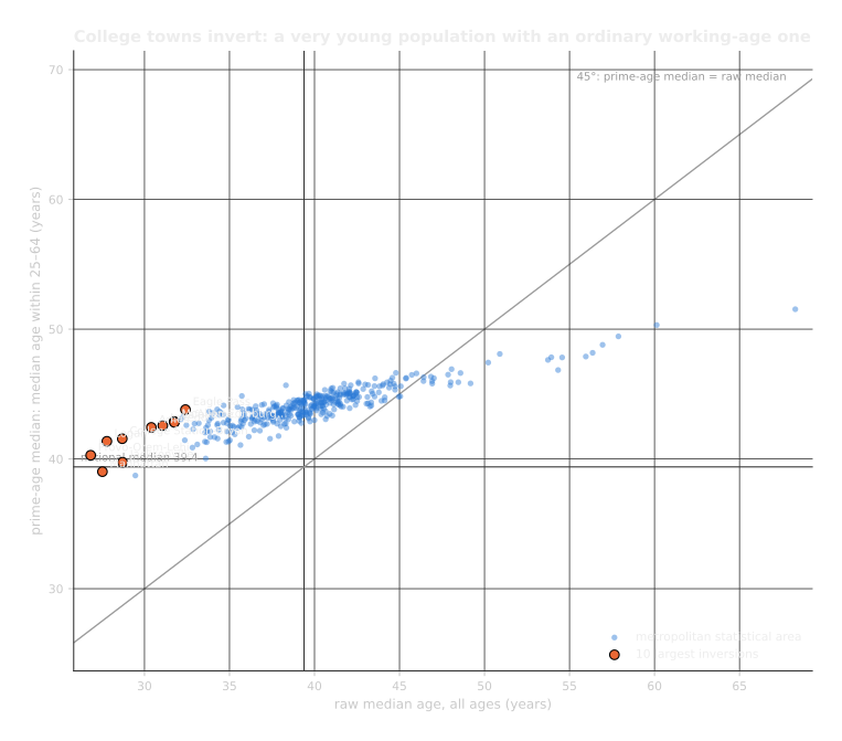
The prime-age median column is the corrective. In the under-100k tier the raw median age and the 25–64 median can differ by more than ten years; a metro can be among the youngest in the country and have an entirely ordinary working-age population.
3. Age-structure typology
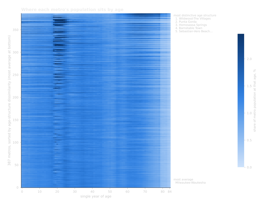
Nine features per metro: modality count on lightly smoothed single-year data, the dissimilarity index, group-quarters share by type (college, military, correctional, nursing), sex ratio at 18–29, and the under-18 and 65+ shares. Standardised, then clustered with both Ward and k-means for k = 6…10 on the 387 metropolitan statistical areas.
Clustering diagnostics
| algorithm | k | silhouette | smallest cluster |
|---|---|---|---|
| ward | 6 | 0.1747 | 1 |
| kmeans | 6 | 0.2174 | 9 |
| ward | 7 | 0.1898 | 1 |
| kmeans | 7 | 0.2167 | 1 |
| ward | 8 | 0.1624 | 1 |
| kmeans | 8 | 0.1941 | 1 |
| ward | 9 | 0.1682 | 1 |
| kmeans | 9 | 0.1992 | 1 |
| ward | 10 | 0.1776 | 1 |
| kmeans | 10 | 0.1991 | 1 |
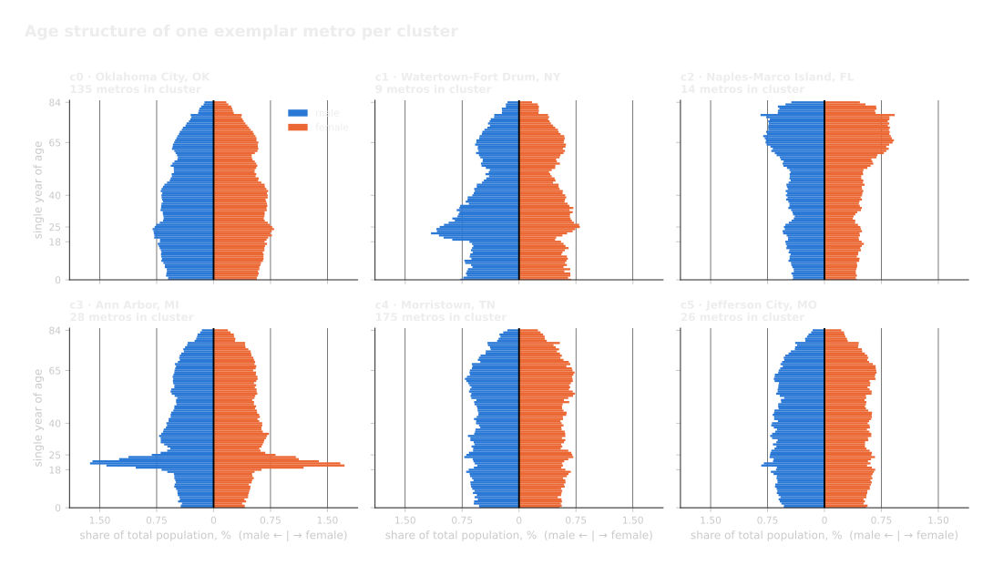
k-means at k=6 scores highest (0.2174); Ward produced a singleton cluster at every k. The two agree on 81.4% of metros at k=6. Silhouette is modest in absolute terms — age structure is continuous, not naturally partitioned — so these clusters are a description, not discovered kinds.
Cluster profiles
| cluster | n | population | median age | modality | dissimilarity | college GQ | military GQ | correctional GQ | sex ratio 18–29 |
|---|---|---|---|---|---|---|---|---|---|
| c0 | 135 | 196.3M | 37.1 | 1.59 | 0.049 | 0.87% | 0.16% | 0.52% | 103.6 |
| c1 | 9 | 1.6M | 33.5 | 1.78 | 0.097 | 0.74% | 4.01% | 0.83% | 143.4 |
| c2 | 14 | 4.5M | 55.1 | 1.64 | 0.199 | 0.34% | 0.21% | 0.89% | 112.8 |
| c3 | 28 | 5.7M | 34.8 | 1.82 | 0.119 | 5.75% | 0.00% | 0.57% | 102.1 |
| c4 | 175 | 82.4M | 41.5 | 2.73 | 0.051 | 0.94% | 0.03% | 0.46% | 103.8 |
| c5 | 26 | 4.9M | 40.0 | 2.42 | 0.046 | 0.74% | 0.18% | 3.36% | 114.5 |
What the data reproduces, and what it does not
Checked against the eight expected types by locating each type’s exemplars. Labels were not forced onto clusters.
| expected type | verdict |
|---|---|
| High fertility | Not separated — falls in c0 |
| College town | Reproduced — all 5 exemplars in c3 |
| Garrison | Partial — 2 of 4 in c1, 2 in c0 |
| Border / agricultural | Not separated — falls in c0 |
| Prime-age magnet | Not separated — falls in c0 |
| Retirement destination | Reproduced — all 3 in c2 |
| Aged in place | Reproduced — all 4 in c4 |
| Near national average | Not separated — falls in c0 |
Four of the eight expected types collapse into a single cluster. High fertility, border/agricultural, prime-age magnet and near-national-average all land together in c0 — Provo–Orem–Lehi (median age 26.8), McAllen (31.7), Austin (35.6) and Columbus OH (37.0) are not separable on age structure alone, though they are young for entirely different reasons. This is not a clustering failure; it is the empirical case for Section 5. If a cross-section could tell these apart, cohort progression would be unnecessary.
The types the data does isolate all have a physical institution or a migration destination behind them. Garrison splits by scale rather than by presence: Jacksonville NC (11.3% military group quarters) and Hinesville (3.2%) form c1, while Clarksville and Killeen–Temple fall into c0 despite comparable barracks populations (5,085 and 9,300 against Hinesville’s 2,977), because their metros are 3.8× and 5.6× larger.
A type the specification placed at county level only appears at metro level. Cluster 5 is 26 metros defined by correctional group quarters at 3.4% of population against 0.5% elsewhere, with a male-skewed sex ratio. The specification expected carceral counties to ‘rarely dominate a whole metro’. On the 2023 delineations they dominate 26:
| metro | correctional GQ share | sex ratio 18–29 | median age |
|---|---|---|---|
| Hanford-Corcoran, CA | 9.0% | 130 | 33.7 |
| Vineland, NJ | 5.5% | 116 | 37.8 |
| Michigan City-La Porte, IN | 4.9% | 124 | 42.0 |
| Carson City, NV | 4.7% | 117 | 43.3 |
| Mansfield, OH | 4.3% | 124 | 41.4 |
| El Centro, CA | 4.1% | 121 | 34.8 |
4. Support and dependency measures
Six measures are computed. Two are absent, and in both cases the only available input would have dated the result:
- Prospective OADR. It needs local life tables by age. The only county-level source, NCHS USALEEP, is a 2010–2015 vintage and excludes Maine and Wisconsin. Pairing it with Vintage 2025 population puts a decade-old mortality regime behind a current numerator, and the threshold ages that fall out of that look far more authoritative than they are.
- Economic support ratio. It needs the National Transfer Accounts age profiles of labour income and consumption, which NTA publishes only through an interactive selection interface with no stable machine-readable endpoint. The profile values are not typed in from memory, so the measure is absent rather than fabricated.
| measure | definition | coverage (of 387 metros) |
|---|---|---|
prime_age_median |
Median age within 25–64 | 387 |
early_career_share |
Pop 25–39 ÷ pop 25–64 | 387 |
oadr |
Pop 65+ ÷ pop 25–64 | 387 |
late_old_ratio |
Pop 75+ ÷ pop 25–64 | 387 |
replacement_ratio |
Pop 20–24 ÷ pop 60–64 | 387 |
admin_support_ratio |
SSA retired workers ÷ QWI employment 25–64 | 369 |
The case for the administrative measure
admin_support_ratio is the most defensible of the six because neither its numerator nor its denominator depends on an age cutoff. The numerator counts people who have actually claimed retired-worker benefits; the denominator counts jobs actually held. Every other measure here inherits an analyst’s decision about where old age begins, and that decision does real work in the ranking.
Its own weaknesses, stated plainly: SSA counts are as of December 2024 against a 7/1/2025 population; small-county figures are rounded to the nearest 5; QWI counts jobs at the workplace, not the worker’s residence, which inflates the denominator for metros that draw commuters; and QWI coverage forces a null for 18 metros rather than an imputed value.
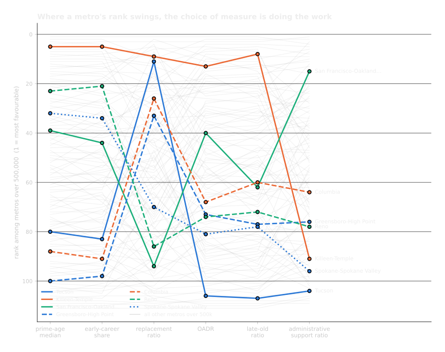
Where a metro’s rank swings across these measures, the choice of measure is doing the work — that is a finding, not noise. San Francisco–Oakland–Fremont climbs from the low 40s on prime-age median to the mid-teens on the administrative ratio; Killeen–Temple falls from 5th to 91st. Anyone ranking metros on ‘dependency’ is choosing an answer when they choose a denominator.
5. Prime-age magnets
The goal is to separate metros that are young because they attract working-age adults from metros that are young because of fertility, institutions, or immigration of young families. All four look alike on median age. They are entirely different economically.
Cohort progression is the evidence
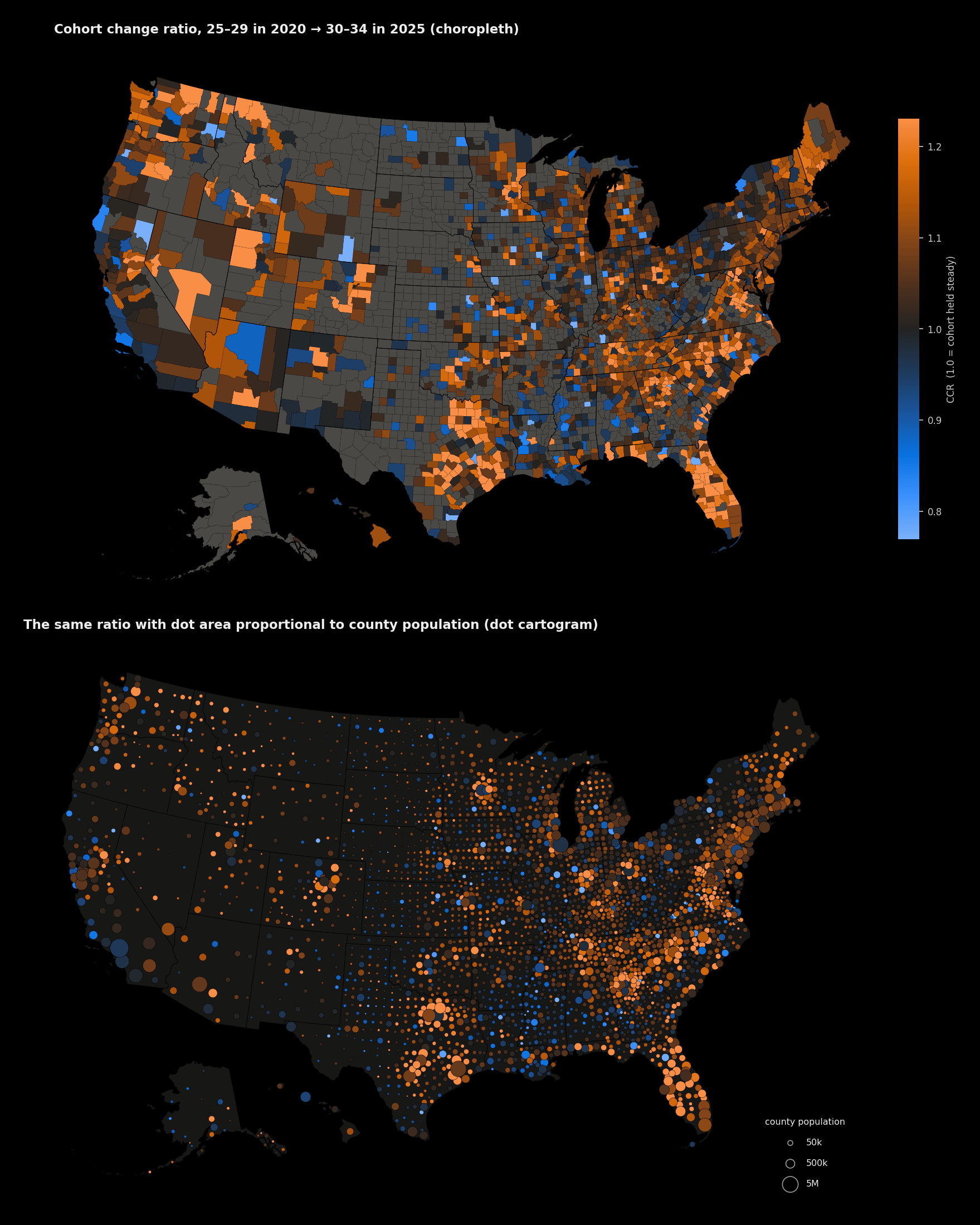
Cohort change ratios compare the same birth cohort at two dates: CCR(a) = P(age a+5, 7/1/2025) ÷ P(age a, 7/1/2020). They are age-specific and require no assumption about where migrants came from, which net-migration totals cannot match.
| diagnostic pair | what it separates | national spread (metros) |
|---|---|---|
ccr_20_24_to_25_29 |
College towns crater; magnets exceed 1.0 | 0.30 – 1.77 (median 1.04) |
ccr_25_29_to_30_34 |
Sustained values above 1.0 are the magnet signature | 0.75 – 1.67 (median 1.03) |
ccr_30_34_to_35_39 |
Retention through family formation | 0.84 – 1.40 (median 1.02) |
ccr_60_64_to_65_69 |
Retirement destinations vs aged-in-place | 0.83 – 1.72 (median 0.93) |
The composite index
| component | weight |
|---|---|
ccr_prime_mean |
0.35 |
early_career_share |
0.15 |
net_domestic_mig_rate |
0.15 |
qwi_emp_25_34_growth |
0.20 |
oadr_inverted |
0.15 |
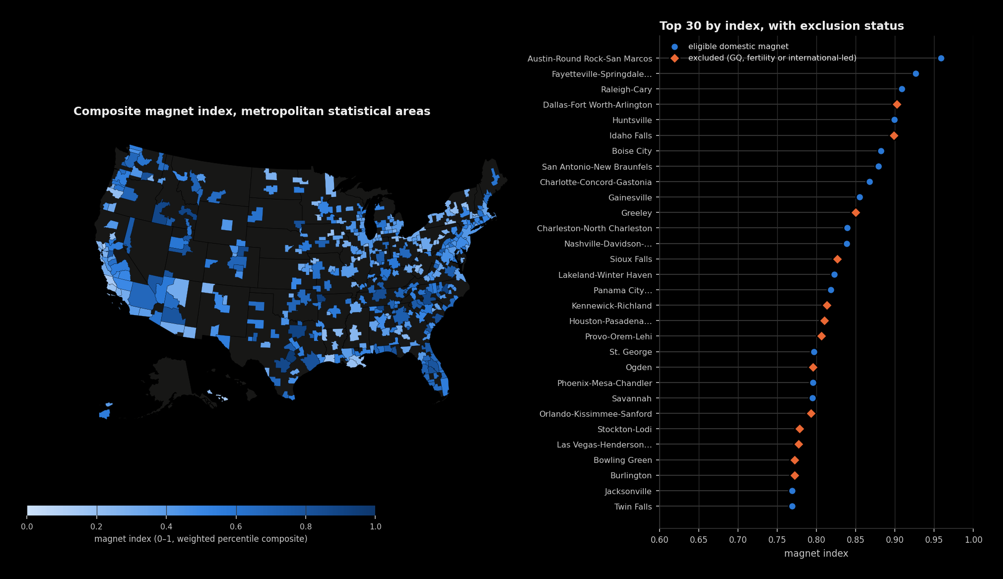
Components enter as percentile ranks rather than z-scores: two of them have long tails that would otherwise let a single extreme metro dominate a standardised average. Weights are a config dict and sensitivity to them is reported below.
Exclusion criteria
None of these deletes a row. A metro that fails a criterion keeps its index value and carries a flag, so the exclusions can be inspected rather than taken on trust.
| criterion | threshold | metros excluded |
|---|---|---|
| Total GQ share at or above the 75th percentile | 0.0376 | 97 |
| College GQ share at or above 2% | 0.02 | 70 |
| Under-5 share in the top decile | 0.0633 | 39 |
| International 50% or more of net migration | 0.50 | 220 |
264 of 387 metros are excluded by at least one criterion, leaving 123 eligible domestic magnets. A further 124 are international-led and are reported as their own group rather than discarded. The international criterion is large by construction: domestic migration is close to zero-sum across metros while international inflow is positive almost everywhere.
Top 20 eligible domestic magnets
| # | metro | index | CCR 25–39 | net domestic migration rate |
|---|---|---|---|---|
| 1 | Austin-Round Rock-San Marcos, TX | 0.9589 | 1.174 | +0.0603 |
| 2 | Fayetteville-Springdale-Rogers, AR | 0.9261 | 1.133 | +0.0786 |
| 3 | Raleigh-Cary, NC | 0.9089 | 1.185 | +0.0704 |
| 4 | Huntsville, AL | 0.8989 | 1.162 | +0.1032 |
| 5 | Boise City, ID | 0.8820 | 1.154 | +0.0911 |
| 6 | San Antonio-New Braunfels, TX | 0.8787 | 1.113 | +0.0515 |
| 7 | Charlotte-Concord-Gastonia, NC-SC | 0.8676 | 1.150 | +0.0504 |
| 8 | Gainesville, GA | 0.8548 | 1.143 | +0.0615 |
| 9 | Charleston-North Charleston, SC | 0.8390 | 1.097 | +0.0667 |
| 10 | Nashville-Davidson–Murfreesboro–Franklin, TN | 0.8387 | 1.073 | +0.0412 |
| 11 | Lakeland-Winter Haven, FL | 0.8229 | 1.323 | +0.1637 |
| 12 | Panama City-Panama City Beach, FL | 0.8180 | 1.221 | +0.1255 |
| 13 | St. George, UT | 0.7969 | 1.177 | +0.1528 |
| 14 | Phoenix-Mesa-Chandler, AZ | 0.7957 | 1.081 | +0.0353 |
| 15 | Savannah, GA | 0.7952 | 1.067 | +0.0439 |
| 16 | Jacksonville, FL | 0.7692 | 1.134 | +0.0738 |
| 17 | Twin Falls, ID | 0.7692 | 1.093 | +0.0487 |
| 18 | Reno, NV | 0.7608 | 1.078 | +0.0330 |
| 19 | Greenville-Anderson-Greer, SC | 0.7554 | 1.116 | +0.0681 |
| 20 | Olympia-Lacey-Tumwater, WA | 0.7543 | 1.090 | +0.0178 |
Sanity checks
Two of the three checks hold exactly. Provo–Orem–Lehi has the lowest median age in the country (26.8) and ranks 19th on the raw index, but its under-5 share exceeds the top-decile threshold, so the fertility exclusion catches it and it is not an eligible magnet. Ithaca, Ames and State College all invert as expected — low raw median age, prime-age median above the national median of 39.4:
| metro | raw median age | prime-age median | inversion |
|---|---|---|---|
| Ithaca, NY | 32.1 | 43.0 | +10.9 |
| Ames, IA | 30.4 | 42.4 | +12.0 |
| State College, PA | 34.0 | 43.5 | +9.5 |
The third check fails for two metros, and the failure is a finding. Austin, Raleigh, Denver, Nashville, Charlotte, Salt Lake City–Murray, Boise, Washington DC and Seattle are all conventionally described as magnets for young workers, and would be expected in the top quintile. Salt Lake City–Murray reaches the 68th percentile and Washington the 45th.
Verified directly against cbsa-est2025-alldata.csv: over 7/1/2020–7/1/2025 the DC metro lost 208,058 net domestic migrants while gaining 262,675 international; Salt Lake City lost 40,598 against +51,256. Seattle (−107,029) and Denver (−33,545) show the same pattern less severely. Weight sensitivity confirms this is not an artefact of the weighting:
| metro | headline weights | equal | CCR only | no domestic migration | migration-heavy |
|---|---|---|---|---|---|
| Austin–Round Rock–San Marcos | 100.0% | 100.0% | 94.3% | 100.0% | 100.0% |
| Raleigh–Cary | 99.5% | 99.0% | 95.1% | 99.2% | 99.2% |
| Boise City | 98.4% | 97.9% | 93.0% | 98.2% | 98.7% |
| Salt Lake City–Murray | 68.2% | 79.8% | 28.9% | 81.1% | 43.2% |
| Washington–Arlington–Alexandria | 45.2% | 47.8% | 44.7% | 57.6% | 26.6% |
Washington never reaches the top quintile under any weighting. Salt Lake City reaches it only when domestic migration is removed entirely, which localises the cause precisely. The index measures domestic attraction, and these two metros did not have it over this window — the conventional expectation encodes a pre-2020 prior. The international-migration exclusion routes both into the international-led group independently, which is where they belong.
The four-way decomposition
Each of the 190 metros below the national median age is assigned a dominant cause. Cause scores are the mean of the percentile ranks of their diagnostics, computed within the below-median set, then normalised to sum to 1.
| cause | metros | population | diagnostic |
|---|---|---|---|
| fertility | 37 | 15.3M | High under-18 share, low CCR(15–19 to 20–24), low net domestic migration |
| institution | 66 | 16.1M | High college+military GQ, sharp 18–24 mode, low CCR(20–24 to 25–29) |
| immigration | 29 | 70.0M | International dominant in net migration, broad 25–49 slab |
| attraction | 58 | 73.6M | High 25–39 CCRs, positive net domestic migration, low GQ share |
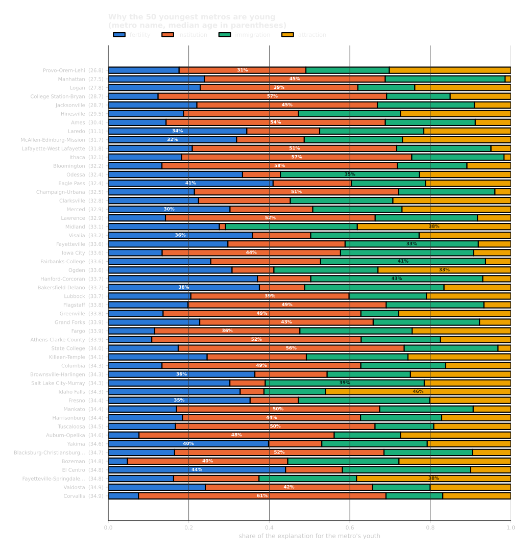
A caveat that changes how the table should be read. The fertility diagnostic is a conjunction: it requires a high under-18 share and a low 18–24 cohort ratio and low net domestic migration. The last two conditions demand the absence of the other causes, so a metro that is genuinely high-fertility and also attracts people cannot score as fertility-dominant.
Provo–Orem–Lehi is the clearest case. Its under-18 share (29.9%) is the highest of any metro below the national median age, but it also gains 20–24-year-olds (CCR 1.52) and domestic migrants (+0.051), so it scores as ‘institution’-dominant at a share of only 0.31 — a genuinely mixed metro rather than a misclassification.
Across all 190 metros the dominant share runs 0.26–0.69 with a median of 0.39. Only 34 metros (18%) have a decisive dominant cause; 25 are near-tied. This is why the figure shows all four contributions rather than a single label — for most metros the argmax alone would be a false precision.
Incidentally, Provo is not the highest under-5 metro in the country:
| metro | under-5 share |
|---|---|
| Hinesville, GA | 8.86% |
| Odessa, TX | 8.65% |
| Eagle Pass, TX | 8.36% |
| Midland, TX | 8.28% |
| Provo-Orem-Lehi, UT | 7.94% |
6. State and county geography
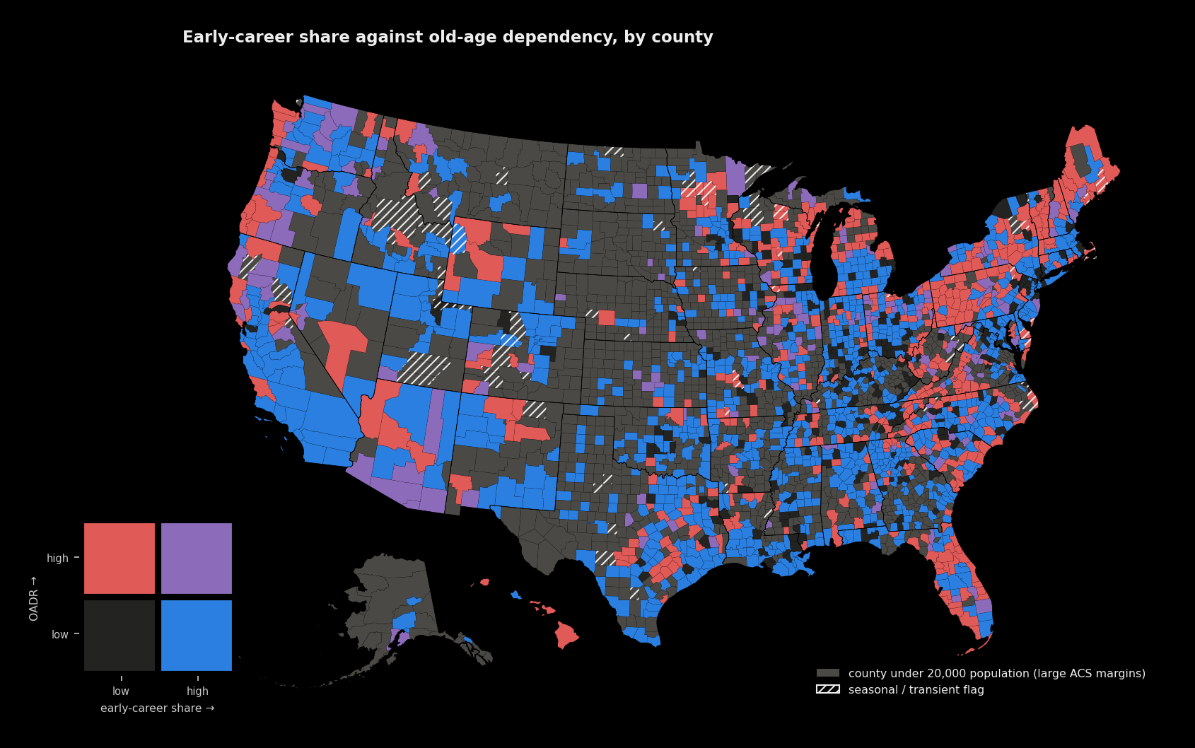
There is deliberately no state choropleth in this report. Florida contains counties younger than the national median, and the same internal spread holds for Texas, California and New York. A state fill would assert a homogeneity the county data contradicts. State results are given as a table with within-state interquartile ranges instead.
Florida makes the point numerically: state median age 43.1, but its counties run from 40.9 at the 25th percentile to 47.8 at the 75th — an interquartile range of 6.9 years, and its youngest county is 33.5.
Full state table with interquartile ranges: figures/state_table.md.
Youngest and oldest states
| state | median age | county p25–p75 | prime-age median | OADR |
|---|---|---|---|---|
| Utah | 32.6 | 33.6–40.2 | 41.8 | 0.266 |
| District of Columbia | 35.0 | 35.0–35.0 | 38.6 | 0.232 |
| Texas | 36.0 | 36.6–43.9 | 42.9 | 0.290 |
| North Dakota | 36.5 | 39.1–45.9 | 42.6 | 0.375 |
| Alaska | 36.7 | 35.9–42.6 | 42.3 | 0.305 |
| Maine | 44.9 | 45.4–49.3 | 45.3 | 0.491 |
| Vermont | 44.4 | 44.9–48.4 | 45.4 | 0.490 |
| New Hampshire | 44.1 | 44.0–49.7 | 45.3 | 0.449 |
| West Virginia | 43.2 | 44.1–47.8 | 45.7 | 0.461 |
| Florida | 43.1 | 40.9–47.8 | 44.9 | 0.456 |
County-level types that rarely dominate a metro
- Carceral counties: 248 counties have correctional group quarters at 5% or more of population together with a male-skewed 18–29 sex ratio. The Census counts incarcerated people at the facility, not their home address, so the age structure of these counties is partly an artefact of enumeration rules. The extreme is Crowley County, Colorado, at 49.9%.
- Seasonal / snowbird counties: 91 counties are flagged, of which 53 also sit in the national top decile for 65+ share. The ACS two-month residence rule partially captures a population that is not present year-round. The flag is built from 2 of the 3 specified signals; H-2A/H-2B certifications were not ingested.
7. Methods, assumptions, and known weaknesses
The framing note: excluding children is an argument, not a cleanup
Several measures here — prime_age_median, early_career_share, oadr, admin_support_ratio — restrict attention to adults and exclude children from both numerator and denominator. This is not a neutral tidying step. The exclusion is a substantive claim.
Children are the largest line item in most local budgets. A metric that drops them ranks a high-fertility metro as unambiguously healthy — few elderly dependents, a thick working-age base — while a municipal public-finance model looking at the same place would score it as high current cost with a deferred and uncertain return, since some share of those children will be educated locally and then leave. Provo–Orem–Lehi and McAllen sit near the favourable end of every adult-only measure in this report and near the demanding end of a school-funding model.
This is stated here rather than left for the metric to assert silently. A reviewer who disagrees with the framing should attack the framing; if it were unstated they would instead attack the definition, and the disagreement would be misdirected.
Group quarters
Group-quarters population is subtracted by age using 2020 Decennial DHC table P18 counts by type, held constant as a share and scaled by county population growth 2020 to 2025. Nationally this is 2.47% of population. The assumption is wrong in specific, knowable ways: a prison that closed or a dormitory that opened between 2020 and 2025 is invisible to it, and the 2020 census GQ count was itself disrupted by the pandemic, which sent a large share of dormitory residents to their family homes on Census Day. That last point biases college-town GQ downward in the base year, so the college adjustment here is if anything conservative.
P18 resolves group quarters to three broad age groups only (under 18, 18–64, 65+), so within a group the subtraction is distributed in proportion to the local age distribution rather than assumed uniform.
The PUMS household-population cross-check specified in the project brief was not performed. It is the one specified validation that is missing, and the discrepancy between the DHC-based subtraction and a direct PUMS household count is therefore unquantified.
Students
Starting the prime-age window at 25 handles most of the college effect. A student-adjusted variant additionally removes ACS college-enrolled 25–34-year-olds. The delta is published as its own column, prime_age_median_student_delta, because its size is the college-town diagnostic rather than a nuisance.
It is negative by construction — removing people from the young end of a 25–64 window can only raise the median. Across metros it runs from -1.93 to -0.17 years (median -0.51). The largest magnitudes are exactly the college towns:
| metro | delta (years) |
|---|---|
| Corvallis, OR | -1.93 |
| Ithaca, NY | -1.85 |
| State College, PA | -1.56 |
| Ann Arbor, MI | -1.55 |
| Bloomington, IN | -1.54 |
| Manhattan, KS | -1.52 |
This variant is deliberately aggressive — graduate students are genuinely resident and often employed — and is computed to measure sensitivity, not because it is the preferred number.
Known weaknesses
Three that are not stated anywhere else in this report:
- Cohort change ratios cannot distinguish migration from mortality or from census-coverage change. At ages 25–39 mortality is small enough that migration dominates, which is why the magnet index uses those cohorts and not older ones.
- The 2020 census base itself carries coverage error, which propagates into every estimate in the series and is not quantified here.
- Connecticut’s group-quarters counts are reallocated from towns to planning regions. That reallocation is exact, but Connecticut is the only state where the geography of the 2020 DHC and the Vintage 2025 estimates disagree, so it is the one place to check first if something looks wrong.
And six stated where they arise, indexed here so this section is still the one place to look:
- Prospective OADR and the economic support ratio are absent, so the seven-measure comparison is a six-measure comparison — Section 4.
- The PUMS household-population validation was not run, so the group-quarters subtraction has no independent check — Section 7, Group quarters.
- QWI counts jobs at the workplace rather than the residence, which biases the administrative support ratio in commuter metros — Section 4.
- SSA county counts are rounded in small counties and predate the population they are divided into — Section 4.
- The seasonal flag uses two of the three specified signals — Section 6.
- Typology silhouette scores are modest, so the clusters describe the data rather than evidencing discrete kinds — Section 3.
8. Data dictionary
Every column in data/processed/. Descriptions are generated from a registry; any column without one is listed explicitly as undocumented rather than omitted.
| table | tag | rows | columns |
|---|---|---|---|
magnets_cbsa.parquet |
mag |
387 | 126 |
measures_cbsa.parquet |
cbsa |
925 | 106 |
measures_county.parquet |
cty |
3,144 | 116 |
measures_state.parquet |
st |
51 | 46 |
typology_cbsa.parquet |
typo |
387 | 17 |
youth_decomposition.parquet |
yd |
190 | 136 |
The in column below gives the tags of the tables carrying that column. A column means the same thing in every table that carries it.
| column | dtype | in | description |
|---|---|---|---|
acs_vintage |
int64 | cty | ACS 5-year vintage actually used (2024, or 2023 on fallback). |
admin_support_available |
bool | mag cbsa cty yd | True where admin_support_ratio could be computed. |
admin_support_ratio |
float64 | mag cbsa cty yd | SSA retired-worker beneficiaries (Dec 2024) ÷ QWI employment aged 25–64 (2025Q1). Null where QWI does not cover every constituent county. |
carceral_flag |
bool | cty | Correctional GQ of 5% or more of population AND sex ratio 18–29 above 110. |
cbsa |
str | mag cbsa typo yd | 5-digit CBSA code, OMB July 2023 delineation. |
cbsa_title |
str | mag cbsa typo yd | CBSA name as published in the Vintage 2025 files. |
ccr_0_4__5_9 |
float64 | mag cbsa cty st yd | Cohort change ratio: population aged 5–9 on 7/1/2025 ÷ population aged 0–4 on 7/1/2020. |
ccr_10_14__15_19 |
float64 | mag cbsa cty st yd | Cohort change ratio: population aged 15–19 on 7/1/2025 ÷ population aged 10–14 on 7/1/2020. |
ccr_15_19__20_24 |
float64 | mag cbsa cty st yd | Cohort change ratio: population aged 20–24 on 7/1/2025 ÷ population aged 15–19 on 7/1/2020. |
ccr_20_24__25_29 |
float64 | mag cbsa cty st yd | Cohort change ratio: population aged 25–29 on 7/1/2025 ÷ population aged 20–24 on 7/1/2020. |
ccr_20_24_to_25_29 |
float64 | mag cbsa cty st yd | Cohort change ratio 20–24 to 25–29 (stable alias of the generated column). |
ccr_25_29__30_34 |
float64 | mag cbsa cty st yd | Cohort change ratio: population aged 30–34 on 7/1/2025 ÷ population aged 25–29 on 7/1/2020. |
ccr_25_29_to_30_34 |
float64 | mag cbsa cty st yd | Cohort change ratio 25–29 to 30–34 (stable alias of the generated column). |
ccr_30_34__35_39 |
float64 | mag cbsa cty st yd | Cohort change ratio: population aged 35–39 on 7/1/2025 ÷ population aged 30–34 on 7/1/2020. |
ccr_30_34_to_35_39 |
float64 | mag cbsa cty st yd | Cohort change ratio 30–34 to 35–39 (stable alias of the generated column). |
ccr_35_39__40_44 |
float64 | mag cbsa cty st yd | Cohort change ratio: population aged 40–44 on 7/1/2025 ÷ population aged 35–39 on 7/1/2020. |
ccr_40_44__45_49 |
float64 | mag cbsa cty st yd | Cohort change ratio: population aged 45–49 on 7/1/2025 ÷ population aged 40–44 on 7/1/2020. |
ccr_45_49__50_54 |
float64 | mag cbsa cty st yd | Cohort change ratio: population aged 50–54 on 7/1/2025 ÷ population aged 45–49 on 7/1/2020. |
ccr_50_54__55_59 |
float64 | mag cbsa cty st yd | Cohort change ratio: population aged 55–59 on 7/1/2025 ÷ population aged 50–54 on 7/1/2020. |
ccr_55_59__60_64 |
float64 | mag cbsa cty st yd | Cohort change ratio: population aged 60–64 on 7/1/2025 ÷ population aged 55–59 on 7/1/2020. |
ccr_5_9__10_14 |
float64 | mag cbsa cty st yd | Cohort change ratio: population aged 10–14 on 7/1/2025 ÷ population aged 5–9 on 7/1/2020. |
ccr_60_64__65_69 |
float64 | mag cbsa cty st yd | Cohort change ratio: population aged 65–69 on 7/1/2025 ÷ population aged 60–64 on 7/1/2020. |
ccr_60_64_to_65_69 |
float64 | mag cbsa cty st yd | Cohort change ratio 60–64 to 65–69 (stable alias of the generated column). |
ccr_65_69__70_74 |
float64 | mag cbsa cty st yd | Cohort change ratio: population aged 70–74 on 7/1/2025 ÷ population aged 65–69 on 7/1/2020. |
ccr_70_74__75_79 |
float64 | mag cbsa cty st yd | Cohort change ratio: population aged 75–79 on 7/1/2025 ÷ population aged 70–74 on 7/1/2020. |
ccr_75_79__80_84 |
float64 | mag cbsa cty st yd | Cohort change ratio: population aged 80–84 on 7/1/2025 ÷ population aged 75–79 on 7/1/2020. |
ccr_prime_mean |
float64 | mag cbsa cty st yd | Mean of CCR(25–29 to 30–34) and CCR(30–34 to 35–39); the magnet signature. |
cluster_kmeans |
int32 | typo | k-means cluster label (k=6); the labels carried forward. |
cluster_ward |
int64 | typo | Ward hierarchical cluster label (k=6). |
contrib_attraction |
float64 | yd | Share of the youth explanation attributed to ‘attraction’; the four sum to 1. |
contrib_fertility |
float64 | yd | Share of the youth explanation attributed to ‘fertility’; the four sum to 1. |
contrib_immigration |
float64 | yd | Share of the youth explanation attributed to ‘immigration’; the four sum to 1. |
contrib_institution |
float64 | yd | Share of the youth explanation attributed to ‘institution’; the four sum to 1. |
county_fips |
str | cty | 3-digit county code within state. |
county_name |
str | cty | County or county-equivalent name. |
dissimilarity |
float64 | mag cbsa cty st typo yd | Age-structure dissimilarity index: half the sum of |p − q| over single-year shares against the nation. |
domestic_magnet_eligible |
bool | mag yd | True where no exclusion criterion fired. |
dominant_cause |
str | yd | Argmax of the four youth-cause scores. Only meaningful alongside dominant_share. |
dominant_share |
float64 | yd | The largest of the four normalised contributions. Near 0.25 means the causes are tied. |
early_career_share |
float64 | mag cbsa cty st yd | Population 25–39 ÷ population 25–64. |
early_career_share_hh |
float64 | mag cbsa cty yd | As above on the household population. |
enrolled_15_17 |
int64 | mag cbsa cty yd | ACS college/graduate enrollment, ages 15 17. |
enrolled_18_24 |
int64 | mag cbsa cty yd | ACS college/graduate enrollment, ages 18 24. |
enrolled_25_34 |
int64 | mag cbsa cty yd | ACS college/graduate enrollment, ages 25 34. |
enrolled_35p |
int64 | mag cbsa cty yd | ACS college/graduate enrollment, ages 35p. |
enrolled_total |
int64 | mag cbsa cty yd | ACS college/graduate enrollment, all ages. |
excl_gq_college |
bool | mag yd | Exclusion criterion ‘gq college’ fired for this metro. |
excl_gq_total |
bool | mag yd | Exclusion criterion ‘gq total’ fired for this metro. |
excl_high_fertility |
bool | mag yd | Exclusion criterion ‘high fertility’ fired for this metro. |
excl_international |
bool | mag yd | Exclusion criterion ‘international’ fired for this metro. |
excluded_any |
bool | mag yd | True where at least one exclusion criterion fired. |
fips |
str | cty | 5-digit county FIPS (state + county). |
gq_all_18_64 |
float64 | mag cbsa cty yd | Group-quarters population of type ‘all’ in age group 18 64, scaled to 2025. |
gq_all_65p |
float64 | mag cbsa cty yd | Group-quarters population of type ‘all’ in age group 65p, scaled to 2025. |
gq_all_u18 |
float64 | mag cbsa cty yd | Group-quarters population of type ‘all’ in age group u18, scaled to 2025. |
gq_college_18_64 |
float64 | mag cbsa cty yd | Group-quarters population of type ‘college’ in age group 18 64, scaled to 2025. |
gq_college_65p |
float64 | mag cbsa cty yd | Group-quarters population of type ‘college’ in age group 65p, scaled to 2025. |
gq_college_share |
float64 | mag cbsa cty typo yd | Group-quarters population of type ‘college’ ÷ total population. |
gq_college_total |
float64 | mag cbsa cty yd | Group-quarters population of type ‘college’, all ages, scaled to 2025. |
gq_college_u18 |
float64 | mag cbsa cty yd | Group-quarters population of type ‘college’ in age group u18, scaled to 2025. |
gq_correctional_18_64 |
float64 | mag cbsa cty yd | Group-quarters population of type ‘correctional’ in age group 18 64, scaled to 2025. |
gq_correctional_65p |
float64 | mag cbsa cty yd | Group-quarters population of type ‘correctional’ in age group 65p, scaled to 2025. |
gq_correctional_share |
float64 | mag cbsa cty typo yd | Group-quarters population of type ‘correctional’ ÷ total population. |
gq_correctional_total |
float64 | mag cbsa cty yd | Group-quarters population of type ‘correctional’, all ages, scaled to 2025. |
gq_correctional_u18 |
float64 | mag cbsa cty yd | Group-quarters population of type ‘correctional’ in age group u18, scaled to 2025. |
gq_imputed |
bool | cty | True where the county had no DHC GQ record and GQ was treated as zero. |
gq_juvenile_18_64 |
float64 | mag cbsa cty yd | Group-quarters population of type ‘juvenile’ in age group 18 64, scaled to 2025. |
gq_juvenile_65p |
float64 | mag cbsa cty yd | Group-quarters population of type ‘juvenile’ in age group 65p, scaled to 2025. |
gq_juvenile_share |
float64 | mag cbsa cty yd | Group-quarters population of type ‘juvenile’ ÷ total population. |
gq_juvenile_total |
float64 | mag cbsa cty yd | Group-quarters population of type ‘juvenile’, all ages, scaled to 2025. |
gq_juvenile_u18 |
float64 | mag cbsa cty yd | Group-quarters population of type ‘juvenile’ in age group u18, scaled to 2025. |
gq_military_18_64 |
float64 | mag cbsa cty yd | Group-quarters population of type ‘military’ in age group 18 64, scaled to 2025. |
gq_military_65p |
float64 | mag cbsa cty yd | Group-quarters population of type ‘military’ in age group 65p, scaled to 2025. |
gq_military_share |
float64 | mag cbsa cty typo yd | Group-quarters population of type ‘military’ ÷ total population. |
gq_military_total |
float64 | mag cbsa cty yd | Group-quarters population of type ‘military’, all ages, scaled to 2025. |
gq_military_u18 |
float64 | mag cbsa cty yd | Group-quarters population of type ‘military’ in age group u18, scaled to 2025. |
gq_nursing_18_64 |
float64 | mag cbsa cty yd | Group-quarters population of type ‘nursing’ in age group 18 64, scaled to 2025. |
gq_nursing_65p |
float64 | mag cbsa cty yd | Group-quarters population of type ‘nursing’ in age group 65p, scaled to 2025. |
gq_nursing_share |
float64 | mag cbsa cty typo yd | Group-quarters population of type ‘nursing’ ÷ total population. |
gq_nursing_total |
float64 | mag cbsa cty yd | Group-quarters population of type ‘nursing’, all ages, scaled to 2025. |
gq_nursing_u18 |
float64 | mag cbsa cty yd | Group-quarters population of type ‘nursing’ in age group u18, scaled to 2025. |
gq_other_inst_18_64 |
float64 | mag cbsa cty yd | Group-quarters population of type ‘other inst’ in age group 18 64, scaled to 2025. |
gq_other_inst_65p |
float64 | mag cbsa cty yd | Group-quarters population of type ‘other inst’ in age group 65p, scaled to 2025. |
gq_other_inst_share |
float64 | mag cbsa cty yd | Group-quarters population of type ‘other inst’ ÷ total population. |
gq_other_inst_total |
float64 | mag cbsa cty yd | Group-quarters population of type ‘other inst’, all ages, scaled to 2025. |
gq_other_inst_u18 |
float64 | mag cbsa cty yd | Group-quarters population of type ‘other inst’ in age group u18, scaled to 2025. |
gq_other_noninst_18_64 |
float64 | mag cbsa cty yd | Group-quarters population of type ‘other noninst’ in age group 18 64, scaled to 2025. |
gq_other_noninst_65p |
float64 | mag cbsa cty yd | Group-quarters population of type ‘other noninst’ in age group 65p, scaled to 2025. |
gq_other_noninst_share |
float64 | mag cbsa cty yd | Group-quarters population of type ‘other noninst’ ÷ total population. |
gq_other_noninst_total |
float64 | mag cbsa cty yd | Group-quarters population of type ‘other noninst’, all ages, scaled to 2025. |
gq_other_noninst_u18 |
float64 | mag cbsa cty yd | Group-quarters population of type ‘other noninst’ in age group u18, scaled to 2025. |
gq_scale_clipped |
bool | cty | True where the growth factor was clipped to [0.5, 2.0]. |
gq_scale_factor |
float64 | cty | 2020 to 2025 population growth factor applied to the GQ counts. |
gq_total_2020 |
float64 | mag cbsa cty yd | Total group-quarters population, 2020 Decennial DHC table P18. |
gq_total_share |
float64 | mag cbsa cty yd | Group quarters ÷ total population. |
hh_pop |
float64 | mag cbsa cty yd | Household population 7/1/2025: total less group quarters scaled to 2025. |
international_led |
bool | mag yd | True where only the international-migration criterion fired. |
intl_share_of_net |
float64 | mag yd | International migration ÷ total net migration, 2020–2025, clipped to [0,1]; 1.0 where net migration is non-positive but international is positive. |
is_metro |
bool | mag cbsa typo yd | True for a metropolitan statistical area, False for micropolitan. |
late_old_ratio |
float64 | mag cbsa cty st yd | Population 75+ ÷ population 25–64. |
lsad |
str | mag cbsa typo yd | Legal/statistical area description (Metropolitan or Micropolitan Statistical Area). |
magnet_index |
float64 | mag yd | Weighted mean of percentile ranks of the five magnet components (0–1). |
magnet_index_partial |
bool | mag yd | True where a component was missing and weights were renormalised. |
magnet_pctile |
float64 | mag yd | Percentile rank on magnet_index. |
magnet_rank |
int64 | mag yd | Rank on magnet_index, 1 = highest. |
magnet_weight_coverage |
float64 | mag yd | Share of the total weight actually available for this metro. |
median_age |
float64 | mag cbsa cty st typo yd | Median age of all ages, linear interpolation within the median single year. |
median_age_county_p25 |
float64 | st | Within-state median age percentile p25 across the state’s counties. |
median_age_county_p75 |
float64 | st | Within-state median age percentile p75 across the state’s counties. |
median_age_hh |
float64 | mag cbsa cty yd | Median age of the household population (group quarters subtracted). |
modality_count |
int64 | typo | Local maxima in the 3-year-smoothed single-year age distribution, prominence 0.12× the mean single-year share. |
mode_sharpness_18_24 |
float64 | mag yd | Mean population share at ages 18–24 ÷ mean share at 30–39. Near 1.0 with no institutional population. |
n_seasonal_signals |
int64 | cty | Count of available signals on which the county is in the top decile. |
n_signals_available |
int64 | cty | How many of the three seasonality signals were available (2 of 3; H-2A/H-2B not ingested). |
net_domestic_mig_2020_2025 |
int64 | mag cbsa yd | Sum of DOMESTICMIG2021…2025 (7/1/2020 to 7/1/2025). |
net_domestic_mig_rate |
float64 | mag cbsa yd | Net domestic migration ÷ 7/1/2020 population. |
net_international_mig_2020_2025 |
int64 | mag cbsa yd | Sum of INTERNATIONALMIG2021…2025. |
net_international_mig_rate |
float64 | mag cbsa yd | Net international migration ÷ 7/1/2020 population. |
oadr |
float64 | mag cbsa cty st yd | Old-age dependency: population 65+ ÷ population 25–64. |
oadr_county_p25 |
float64 | st | Within-state oadr percentile p25 across the state’s counties. |
oadr_county_p75 |
float64 | st | Within-state oadr percentile p75 across the state’s counties. |
oadr_hh |
float64 | mag cbsa cty yd | As above on the household population. |
prime_age_median |
float64 | mag cbsa cty st yd | Median age within the 25–64 population. |
prime_age_median_county_p25 |
float64 | st | Within-state prime age median percentile p25 across the state’s counties. |
prime_age_median_county_p75 |
float64 | st | Within-state prime age median percentile p75 across the state’s counties. |
prime_age_median_hh |
float64 | mag cbsa cty yd | Prime-age median on the household population. |
prime_age_median_student_adj |
float64 | mag cbsa cty yd | Prime-age median after also removing ACS college-enrolled 25–34. |
prime_age_median_student_delta |
float64 | mag cbsa cty yd | prime_age_median_hh minus prime_age_median_student_adj. NEGATIVE by construction; the magnitude is the college-town diagnostic. |
qwi_amplitude |
float64 | cty | (max − min) ÷ mean of the four 2024 quarterly all-ages QWI employment values. |
qwi_emp_25_34_2020 |
float64 | mag cbsa cty yd | QWI employment aged 25–34, 2020Q1. |
qwi_emp_25_34_2025 |
float64 | mag cbsa cty yd | QWI employment aged 25–34, 2025Q1. |
qwi_emp_25_34_growth |
float64 | mag cbsa cty yd | Ratio of the two preceding columns. |
qwi_emp_25_64 |
float64 | mag cbsa cty yd | LEHD QWI employment aged 25–64, 2025Q1 (sum of bands A04–A07). |
rank_ccr_prime_mean |
float64 | mag yd | Percentile rank of ccr prime mean used as a magnet-index component. |
rank_early_career_share |
float64 | mag yd | Percentile rank of early career share used as a magnet-index component. |
rank_net_domestic_mig_rate |
float64 | mag yd | Percentile rank of net domestic mig rate used as a magnet-index component. |
rank_oadr_inverted |
float64 | mag yd | Percentile rank of oadr inverted used as a magnet-index component. |
rank_qwi_emp_25_34_growth |
float64 | mag yd | Percentile rank of qwi emp 25 34 growth used as a magnet-index component. |
replacement_ratio |
float64 | mag cbsa cty st yd | Population 20–24 ÷ population 60–64. |
retired_workers |
float64 | mag cbsa cty yd | SSA retired-worker beneficiaries, December 2024. |
score_attraction |
float64 | yd | Raw cause score for ‘attraction’: mean of the percentile ranks of its diagnostics. |
score_fertility |
float64 | yd | Raw cause score for ‘fertility’: mean of the percentile ranks of its diagnostics. |
score_immigration |
float64 | yd | Raw cause score for ‘immigration’: mean of the percentile ranks of its diagnostics. |
score_institution |
float64 | yd | Raw cause score for ‘institution’: mean of the percentile ranks of its diagnostics. |
seasonal_flag |
bool | mag cbsa cty yd | True where the county is in the top decile of at least two available seasonality signals. |
seasonal_housing_share |
float64 | cty | Seasonal/occasional-use housing units ÷ total housing units (ACS B25004_006 ÷ B25001_001). |
sex_ratio_18_29 |
float64 | mag cbsa cty st typo yd | Males per 100 females aged 18–29. |
share_0_17 |
float64 | mag cbsa cty st typo yd | Population aged 0–17 ÷ total population. |
share_18_24 |
float64 | mag cbsa cty st yd | Population aged 18–24 ÷ total population. |
share_25_39 |
float64 | mag cbsa cty st yd | Population aged 25–39 ÷ total population. |
share_25_49 |
float64 | mag yd | Population 25–49 ÷ total population. |
share_40_64 |
float64 | mag cbsa cty st yd | Population aged 40–64 ÷ total population. |
share_65_74 |
float64 | mag cbsa cty st yd | Population aged 65–74 ÷ total population. |
share_65p |
float64 | typo | Population 65+ ÷ total population. |
share_75p |
float64 | mag cbsa cty st yd | Population aged 75 and over ÷ total population. |
share_under5 |
float64 | mag cbsa cty st yd | Population under 5 ÷ total population. |
snowbird_flag |
bool | cty | Seasonal flag set AND 65+ share in the national top decile. |
ssa_year |
int64 | cty | SSA data year (2024). |
state_fips |
str | cty st | 2-digit state FIPS. |
state_name |
str | cty st | State name. |
top_decile_qwi_amplitude |
bool | cty | True where the county is in the top decile of qwi amplitude. |
top_decile_seasonal_housing_share |
bool | cty | True where the county is in the top decile of seasonal housing share. |
total_pop |
float64 | mag cbsa cty st typo yd | Total resident population, 7/1/2025 estimate. |
total_pop_2020 |
float64 | mag cbsa cty st yd | Total resident population, 7/1/2020 estimate (YEAR index 2). |
Every column in every processed table carries a description.
Appendix: source inventory
80 cached files, 251 MB. Full URLs, byte sizes, SHA256 hashes and retrieval timestamps are in data/raw/MANIFEST.md; every HTTP request with its status code is logged in data/raw/fetch_log.jsonl.
| source | status |
|---|---|
acs_b01001_county — ACS 5-year B01001 — sex by age, county cross-check |
available |
acs_b01003_tract_pop — ACS 5-year B01003 — tract population, weights for USALEEP county aggregation |
available |
acs_b14004_county — ACS 5-year B14004 — college enrollment by age, county |
available |
acs_b25004_county — ACS 5-year B25004 — vacancy status incl. seasonal use |
available |
acs_b26001_county — ACS 5-year B26001 — group quarters population total |
available |
dhc_p18_gq_county — 2020 Decennial DHC P18 — GQ by sex x age x type, county |
available |
qwi_employment_county — LEHD QWI — employment by county, worker age band, 2020Q1/2025Q1 + 2024 quarterly |
available |
ssa_retired_workers_county — SSA OASDI — retired-worker beneficiaries by county, Dec 2024 (via Wayback; ssa.gov 403s non-browser clients) |
available |
usaleep_tract_lifetables — NCHS USALEEP — abridged life tables e(x) by census tract, 2010-2015 |
available |
Reproduce with make all. Nothing under data/raw/ is re-downloaded if it is already present.